

Different protein foundation models learn fundamentally different signals from their training data. Sequence models like the ESM family learn which mutations look evolutionarily plausible across millions of proteins. MSA-based models capture how residues co-evolve within a specific protein family. Structure models like AlphaFold and Protenix learn the geometric constraints of how a chain folds in 3D space.
Successful molecular design requires getting all of these aspects right simultaneously.
One way the field has tried to solve this is through monolithic pre-training: either forcing a single giant model to learn sequence and structure together from scratch (like ESM3), or scaling sequence models to tens of billions of parameters (like ProGen3). Both approaches have hit a scaling wall on downstream fitness prediction. Forcing multiple modalities into one pre-training objective often compromises representation quality per parameter, and brute-force parameter scaling yields sharply diminishing returns when predicting subtle mutational effects on benchmarks like ProteinGym.
Specialized models still capture the sharpest signals-they just hold that knowledge in isolated, incompatible latent spaces.
At the same time, supervised protein engineering always operates in a sparse data regime. Even a large wet-lab screen only ever samples a tiny fraction of combinatorial sequence space. To extract the most signal from sparse experimental datasets without hitting the pre-training scaling wall, we asked a different question:
Instead of training one giant model to do everything, what if we keep specialized models frozen and teach them to translate what they know into a shared latent space?
We call this approach Protein Fuse: a framework that connects frozen protein models through lightweight latent translators, combining complementary sequence, structural, and evolutionary information for fitness prediction.
Translating two models’ latent spaces
Every protein model maps its inputs into an internal representation - an embedding - shaped by its architecture, training data, and learning objective. Even when two models capture overlapping biological signal about the same protein, they encode it in completely different coordinate systems.
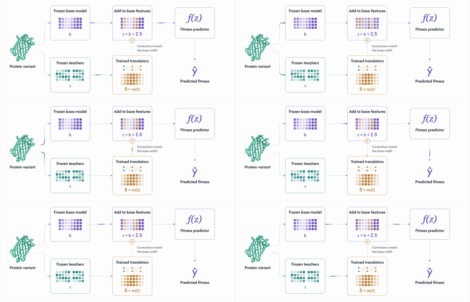
To combine these learnings, we pick one model to improve and let the others feed it what they know. We call the model being improved the base, and the models feeding it information to the teacher. A teacher model doesn’t have to be better than the base model on its own. It just needs to know something the base doesn’t. But each model has their own embeddings in latent space. Even the same knowledge is represented differently, so we need a translator that carries each teacher’s representation into the base model’s space.1
Here’s how it looks: we run one protein variant through the base model and the teacher models, all frozen. Each teacher’s features pass through a small translator that turns them into corrections. These corrections get added to the base model’s features, and a predictor reads the combined result to estimate the protein fitness.
How do we know it’s working?
We evaluated this set-up on the Sarkisyan avGFP dataset2 from ProteinGym. GFP is one of the most studied proteins and an industry-standard benchmark for fitness prediction. Every variant in the dataset has a measured brightness. The model trains on a subset of these labelled variants and has to predict fitness across the held-out set.3
In protein design, what matters most is ranking. Learning effectively from sparse datasets unlocks the ability to explore wider regions of sequence space and reliably surface the highest-performing variants at the top of the distribution. We score this ranking accuracy with Spearman correlation.
To test whether a model is learning transferable biology rather than just memorizing local positions, ProteinGym hides the test data in three ways:
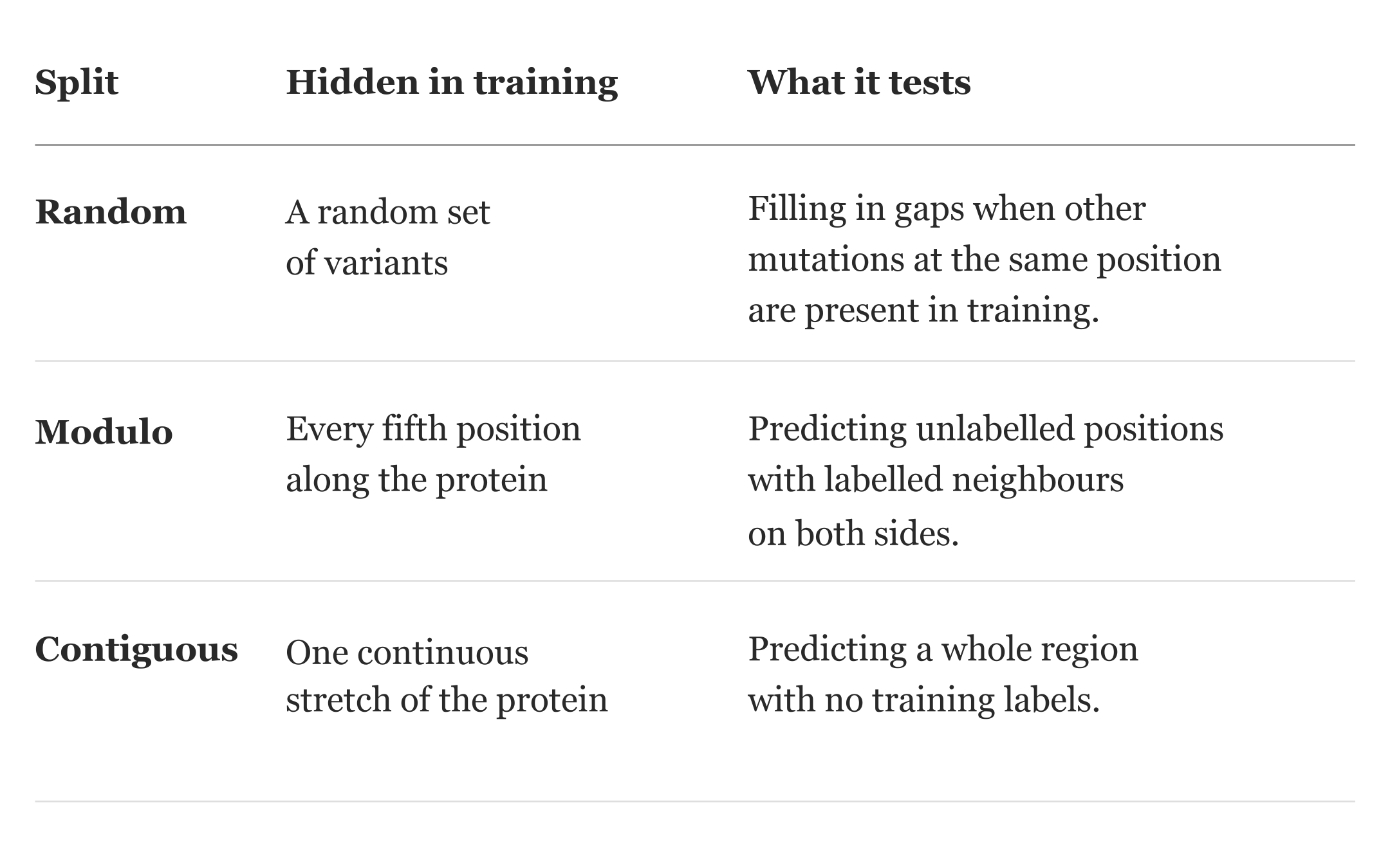
Each split is run across five folds, hiding a different fifth of the data each round. Our headline score is the average across all three split schemes.4 Contiguous is the hardest of the three because it tests how well a model generalizes into unmapped regions of a protein, and surprisingly, that is where latent translation helped the most.
Putting the models together
In our in-house supervised evaluation, we first benchmarked ten models on their own. Standalone Protenix was strongest (Spearman 0.5737), followed by MSA Transformer (0.5342) and ESM-C 600M, layer 12 (0.4060). The other single-sequence models scored between 0.3324 and 0.3956. Prediction heads differed across these standalone evaluations. After adding teachers, however, the Protenix-based system did not outperform the MSA Transformer-based system, so we chose MSA Transformer as the final base.
For our final architecture, we paired MSA Transformer as the base model with two complementary teachers: ESM-C (extracting per-residue features at the mutated position) and Protenix (extracting two summary statistics of how residue pairs relate). We stop Protenix in its trunk before it folds a full 3D structure, since all we need is its internal pairwise representation of the protein.
The most direct baseline for combining these features is concatenation: run every model, place their feature vectors side by side, and train a regressor on the combined vector. Nothing is translated. The predictor simply sees: [MSA features ; ESM-C features; Protenix features] and has to learn which coordinates matter.
Representation transfer is different. Teacher features are not appended to the base vector. Each teacher block first passes through a small MLP mapper, and the mapper outputs a correction with the same width as the base representation. Those corrections are added to the MSA vector, giving a new MSA-shaped vector for the fitness predictor to read:
translated MSA vector = original MSA vector + mapped teacher corrections
This is the core architectural difference: concatenation forces the final regressor to reconcile several high-dimensional feature spaces at once from sparse labels, while representation transfer projects the teachers’ structural and sequence signals into the base model’s coordinate space before prediction.
We tried two ways to train that mapper.
1. Embedding reconstruction
Our first pilot trained the mapper to directly recreate the base model’s embedding from a teacher’s embedding for the same GFP variant - rewarding the mapper whenever m(t) looked like b.
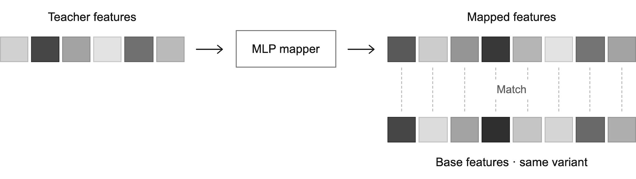
This served as a clean sanity check: if a small MLP can reconstruct one model’s embedding from another, the two latent spaces clearly share structure. However, the objective has a built-in ceiling: it only asks the mapper to copy what MSA Transformer already encoded. Whenever ESM-C or Protenix captures fitness-relevant structural or sequence signals that are weak in the original MSA vector, pure reconstruction has no incentive to preserve it.
2. Predictor-guided transfer
Our final method replaces reconstruction with predictor-guided transfer. Here, the mapper is no longer trained to copy the MSA embedding - it is trained to produce a residual correction that directly improves GFP fitness predictions.5
We first train Support Vector Regressors (SVR guides, q) strictly on the original MSA features and freeze them. During mapper training, the translated MSA-shaped vector passes through one of these frozen guides. When the guide’s fitness prediction is off, the error is backpropagated through the frozen guide and into the mapper. The SVR guide remains fixed, and MSA Transformer, ESM-C, and Protenix stay completely frozen; only the mapper weights θ update.6
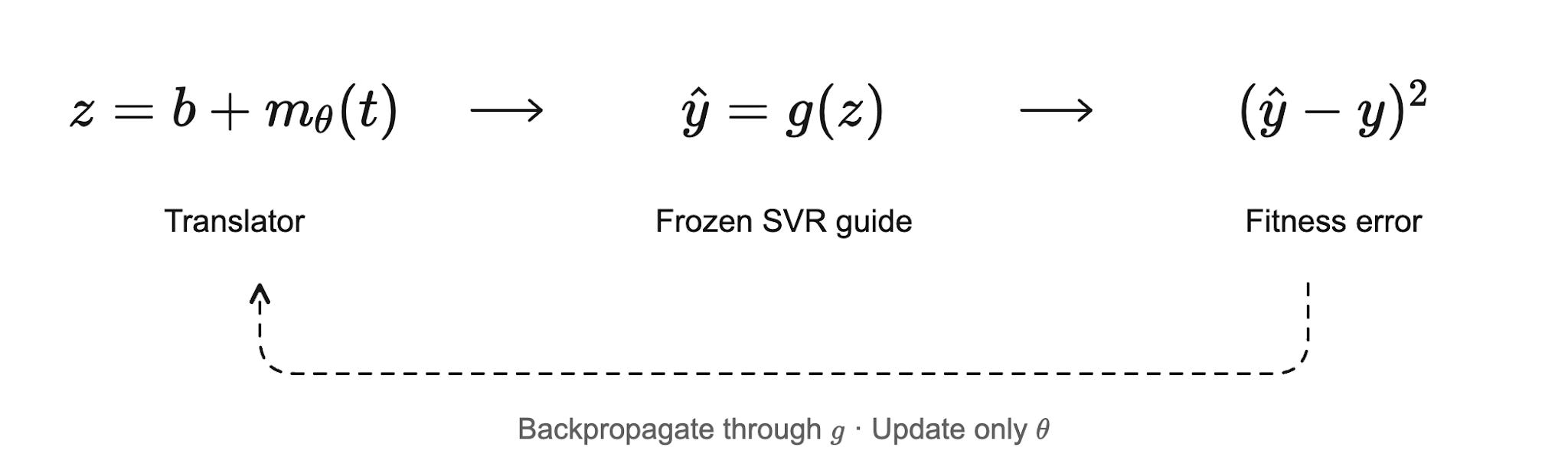
Once mapper training converges, we discard the frozen guides, generate the translated vectors with the trained mapper, and fit a fresh evaluation SVR on those vectors for held-out predictions. Because the guide q was frozen on the original MSA space, it acts as a regularizer: it forces the mapper to extract only the structural and sequence signals from Protenix and ESM-C that align with fitness-relevant directions in the base space, rather than overfitting to local sequence positions.
How well does it work?
With predictor-guided transfer, our overall score rose to 0.6433, up from our in-house MSA Transformer baseline of 0.5342 and ahead of standalone Protenix (0.5737). Separately, the best official ProteinGym supervised GFP entry in the results we consulted is TranceptEVE + one-hot encoding at 0.529; the official MSA Transformer embedding result is 0.512. We also compared the translator directly against concatenating all three models’ features together. The strongest version of concatenation (using block-normalized features) scored 0.6308.
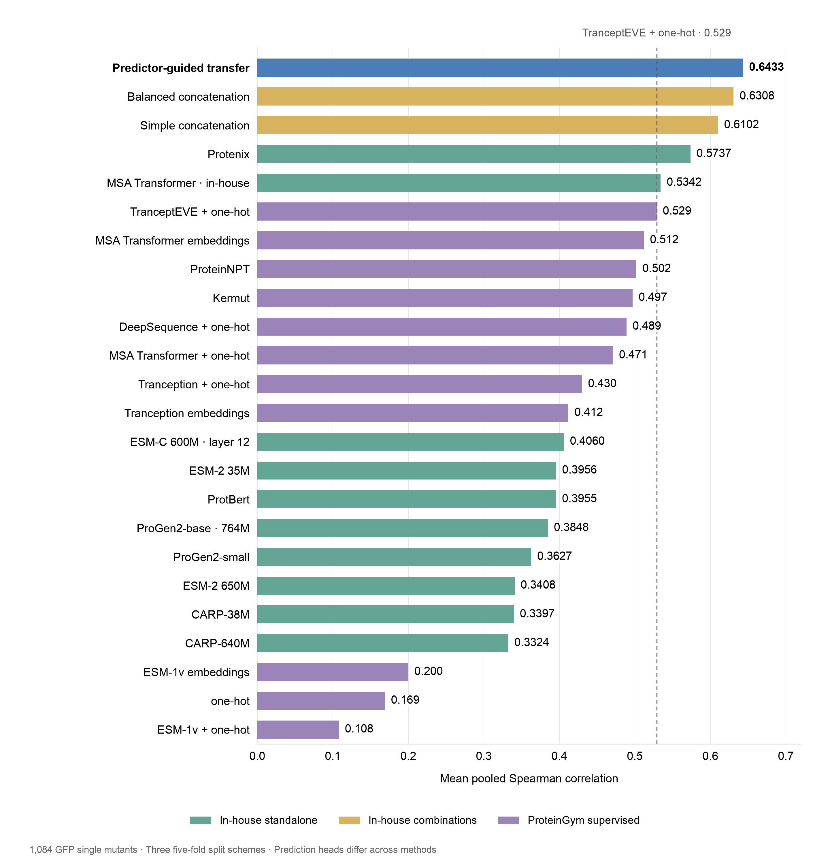
Supervised prediction on 1,084 GFP single mutants: mean pooled Spearman across the random, modulo and contiguous five-fold splits. In-house standalone models use different prediction heads: selected SVRs, SVR + MLP ensembles, or earlier nested head selection. Transfer and concatenation use inner-selected SVRs and one initialization seed. Public baselines are from ProteinGym. Dashed line: TranceptEVE + one-hot (0.529). “One-hot” encodes each amino acid with one 1 and zeros elsewhere. Scores compare complete prediction pipelines, not encoders alone.
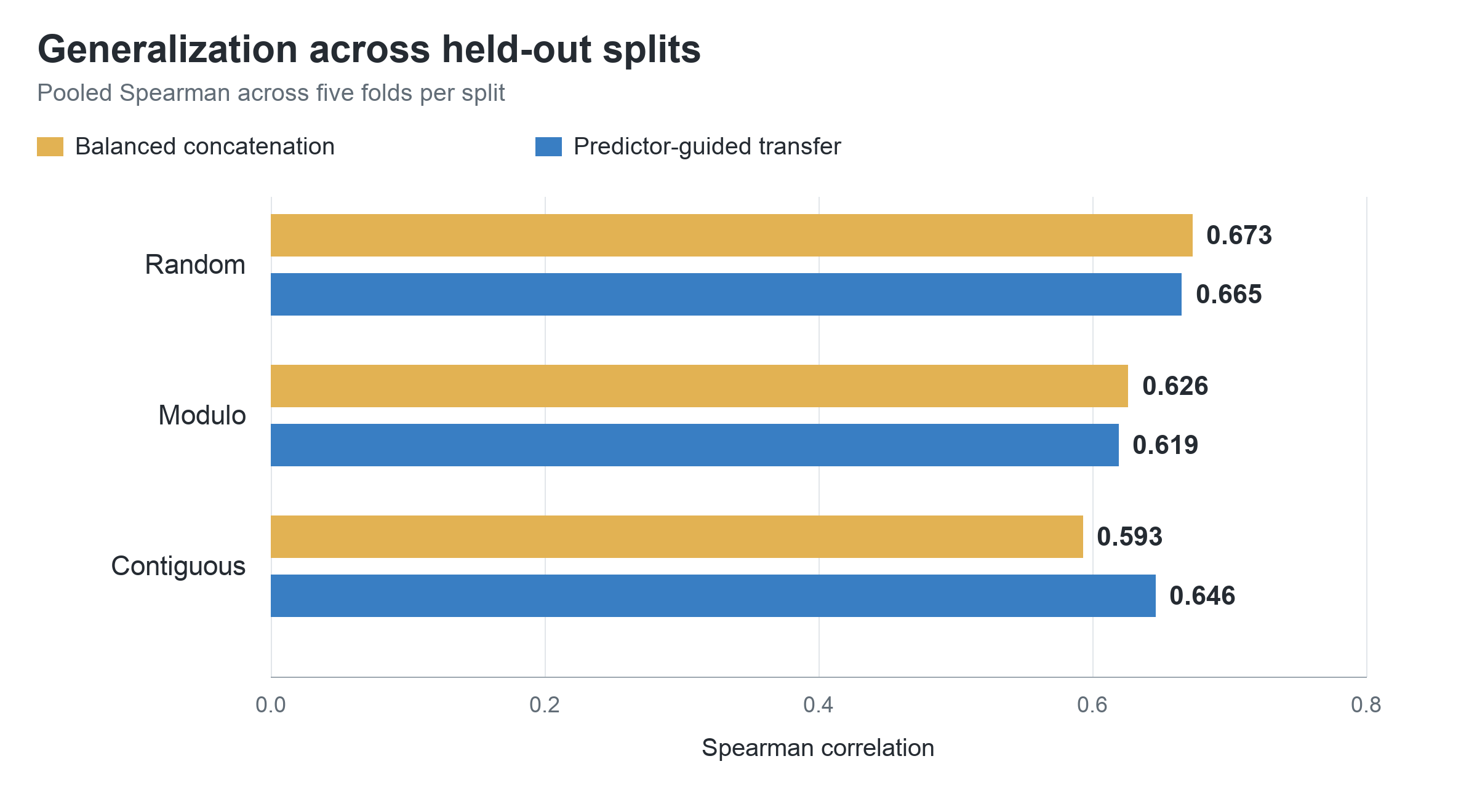
Each bar pools the five held-out folds within one split scheme. Both methods use the same Protenix and ESM-C teacher features. Predictor-guided transfer leads on contiguous regions; balanced concatenation leads on random and modulo splits.
Adding the teacher models drives the bulk of the overall improvement: even concatenating their features with the base model lifts the headline score from 0.5342 to 0.6308.
The translator adds a smaller gain on top of that, and it shows up most clearly on the contiguous split, where a protein is hidden during training. The translator scored 0.646 against 0.593 for concatenation, and it came out ahead in all five rounds. So the model seems to learn more about protein biochemistry when we translate the teachers’ features instead of just combining them compared to other methods.
Latent fusion can enable learning from sparse datasets
There are already many strong protein models, with new ones arriving almost every month, each trained on a different modality or objective. As monolithic efforts like ESM3 and ProGen3 have shown, simply scaling parameter counts or cramming sequence and structure into a single pre-training objective hits diminishing returns on downstream fitness prediction.
For protein design, most workflows either pick a single specialist model or concatenate embeddings from a few models into an increasingly wide vector. This work points to another path: keep specialized models frozen and train lightweight translators that project what they’ve learned into a shared latent space.
On GFP, training a few small residual translators on fewer than a thousand labelled variants lifted our ranking correlation from our in-house MSA Transformer baseline of 0.5342 to 0.6433, surpassing both the strongest standalone model in our evaluation (0.5737 for Protenix) and block-normalized feature concatenation (0.6308).
The result we care about most is performance on unseen regions. Real-world protein engineering constantly moves into unmapped territory - redesigning a loop, reshaping a binding surface, or modifying domains where no prior mutational measurements exist. That is exactly where latent translation helped most, beating concatenation across every contiguous fold (0.646 vs. 0.593).
Extracting more generalizable signal from sparse datasets unlocks the ability to explore much wider regions of sequence space. Rather than waiting on larger monolithic models, getting specialized models to share what they already know gives us a fast, sample-efficient way to generalize into new regions of a protein and make sharper design calls.
The Protein Fuse training and evaluation code is now available on GitHub. The README explains how to generate embeddings with the upstream models, export them in the required format, and run the downstream experiments. Precomputed embeddings and upstream extraction scripts are not included. We invite researchers to extend the approach to larger datasets, additional proteins, and other model combinations, and evaluate where the gains persist.
Citing Protein Fuse
If you use Protein Fuse in your research or build on this implementation, please cite:
Mandrake Bio. (2026). Protein Fuse: Teaching Protein Models to Talk to Each Other. The Assay.
@misc{mandrake2026proteinfuse,
  author       = {{Mandrake Bio}},
  title        = {{Protein Fuse}: Teaching Protein Models to Talk to Each Other},
  year         = {2026},
  howpublished = {The Assay},
  url          = {https://research.mandrake.bio/p/protein-fuse-teaching-protein-models}
}
Code: github.com/MandrakeBio/Protein-Fuse
For reproducibility, please also report the commit hash of the code used in your experiments.
The processed full assay contains 51,714 variants. Our main benchmark uses its 1,084 single mutants: each sequence differs from the reference at one amino-acid position. The remaining 50,630 variants have multiple substitutions and form a different evaluation problem.
ProteinGym has two benchmarks. In the zero-shot one, a model predicts without seeing any measured data for the protein. In the supervised one, it first learns from some measured variants. We used the supervised one, with all the big models kept frozen.
The benchmark is ProteinGym’s Sarkisyan avGFP set (1,084 single mutants), scored as the mean of pooled Spearman correlations over the official random, modulo and contiguous five-fold splits. The full technical write-up, with every control and the complete results table, is available on request.
To stop the translator from memorising answers, each guide is trained on one part of the training data and only judges variants from a different part.